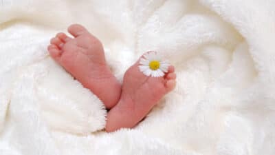
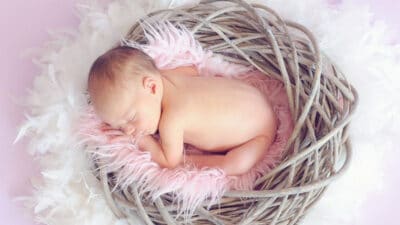
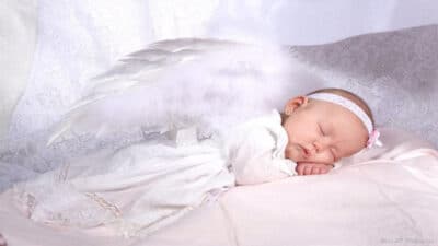
Table of Contents
Local linearity means just what it says. A function is locally linear over an interval iff that interval is sufficiently small for a tangent line to closely approximate the function over the interval.
What is local linearity used for?
Sal introduces the idea of approximating curves using their tangent line equations. This is also called “local linearization.”.
What is the principle of local linearity?
The principle of local linearity tells us that if we zoom in on a point where a function y=f(x) y = f ( x ) is differentiable, the function will be indistinguishable from its tangent line.
What is local linear approximation?
The idea behind local linear approximation, also called tangent line approximation or Linearization, is that we will zoom in on a point on the graph and notice that the graph now looks very similar to a line.
How do you know if a function is locally linear?
We simply say “f is locally linear” (or “differentiable”) if it’s locally linear at all points in a specified domain. x = a. So: “y = f(x) is locally linear, or differentiable, at the point x = a” simply means “the derivative f/(a) exists.”.
How do you find LX?
Use the formula L(x)=f(a)+f'(a)(x−a) to get L(x)=4+18(x−16)=18x+2 as the linearization of f(x)=x12 at a=16 .
How do you know if approximation is over or underestimate?
If the graph is concave down (second derivative is negative), the line will lie above the graph and the approximation is an overestimate.
What is local linearization of a function at a point?
Fundamentally, a local linearization approximates one function near a point based on the information you can get from its derivative(s) at that point. In the case of functions with a two-variable input and a scalar (i.e. non-vector) output, this can be visualized as a tangent plane.
Is linear approximation the same as linearization?
Linear approximation, or linearization, is a method we can use to approximate the value of a function at a particular point. The reason liner approximation is useful is because it can be difficult to find the value of a function at a particular point. Square roots are a great example of this.
What are the different ways of approximation?
Approximate methods may be divided into three broad interrelated categories; “iterative,” “asymptotic,” and “weighted residual.” The iterative methods include the development of series, methods of successive approximation, rational approximations, and so on.
What is linearization in Calc?
The Linearization of a function f(x,y) at (a,b) is L(x,y) = f(a,b)+(x−a)fx(a,b)+(y−b)fy(a,b). This is very similar to the familiar formula L(x)=f(a)+f′(a)(x−a) functions of one variable, only with an extra term for the second variable.
What is the instantaneous rate of change of a function?
The instantaneous rate of change is the slope of the tangent line at a point. A derivative function is a function of the slopes of the original function.
How do you know if a derivative is concave up or down?
Taking the second derivative actually tells us if the slope continually increases or decreases. When the second derivative is positive, the function is concave upward. When the second derivative is negative, the function is concave downward.
How are Linearizations used?
In the study of dynamical systems, linearization is a method for assessing the local stability of an equilibrium point of a system of nonlinear differential equations or discrete dynamical systems. This method is used in fields such as engineering, physics, economics, and ecology.
Which theorem is used in linearization?
A basic contribution to the linearization problem for autonomous differential equations is the Hartman–Grobman theorem (see [6] and [7]).
Why is linearization important?
Linearization is important because linear functions are easier to deal with. Using linearization, one can estimate function values near known points. JUSTIFYING THE LINEAR APPROXIMATION. If the second variable y = y0 is fixed, then we have a one-dimensional situation where the only variable is x.
Is overestimate concave up or down?
If the tangent line between the point of tangency and the approximated point is below the curve (that is, the curve is concave up) the approximation is an underestimate (smaller) than the actual value; if above, then an overestimate.)Oct 24, 2012.
How do you know if trapezoidal sum is an over or underestimate?
You still use the formula to find the width of the trapezoids. NOTE: The Trapezoidal Rule overestimates a curve that is concave up and underestimates functions that are concave down.
Is concave up over or underestimate?
Function is always decreasing → LEFT is an overestimate, RIGHT is an underestimate. Function is always concave up → TRAP is an overestimate, MID is an underestimate.
How do you find the local linearization at a point?
Explanation: The linearization of a differentiable function f at a point x=a is the linear function L(x)=f(a)+f'(a)(x−a) , whose graph is the tangent line to the graph of f at the point (a,f(a)) . When x≈a , we get the approximation f(x)≈L(x) .
How does local linearity contribute to the definition of a function’s derivative?
Certain graphs, specifically those that are differentiable, have a property called local linearity. Functions that are differentiable at a point are locally linear there and functions that are locally linear are differentiable. In the next post we will see how to use the local linear idea to introduce the derivative.
What is linearization in network security?
In cryptography, the extended Sparse Linearization (XSL) attack is a method of cryptanalysis for block ciphers. In the XSL attack, a specialized algorithm, termed extended Sparse Linearization, is then applied to solve these equations and recover the key.
What is linear approximation of a function?
In mathematics, a linear approximation is an approximation of a general function using a linear function (more precisely, an affine function). They are widely used in the method of finite differences to produce first order methods for solving or approximating solutions to equations.
Is tangent line and linearization the same?
It is exactly the same concept, except brought into R3. Just as a 2-d linearization is a predictive equation based on a tangent line which is used to approximate the value of a function, a 3-d linearization is a predictive equation based on a tangent plane which is used to approximate a function.
How do you do linear approximation in fxy?
The linear approximation of f(x, y) at (a, b) is the linear function L(x, y) = f(a, b) + fx(a, b)(x – a) + fy(a, b)(y – b) . The linear approximation of a function f(x, y, z) at (a, b, c) is L(x, y, z) = f(a, b, c) + fx(a, b, c)(x – a) + fy(a, b, c)(y – b) + fz(a, b, c)(z – c) .